Simple Linear Regression
Simple linear regression is a supervised learning algorithm that fits a straight line through data with one input feature, so it can predict a continuous output.
Your Path Through This Lesson
0 of 5 done
- Explain what the best-fit line minimises.
- Calculate a slope and an intercept by hand.
- Fit, read and use
LinearRegressionin scikit-learn.
The Idea: Draw the Best Line
Let's go back to our five students:
| Hours studied () | Marks () |
|---|---|
| 1 | 20 |
| 2 | 40 |
| 3 | 50 |
| 4 | 40 |
| 5 | 50 |
Plot them and you'll see the marks go up with hours, but the points don't sit on a perfect line. Real data never does. So the question becomes: which straight line passes as close as possible to all the points? That line is called the best-fit line, and finding it is all simple linear regression does.
Writing the Line Three Ways
You learned the equation of a line in school. Machine learning writes the same line with different letters, and you'll see all three versions in books, so let's line them up:
| Where you see it | Equation | Intercept | Slope |
|---|---|---|---|
| School maths | |||
| Statistics | |||
| Machine learning |
We'll use the machine learning version:
- is the hypothesis: the model's prediction for input . It's the same thing as .
- (theta zero) is the intercept: the prediction when , where the line crosses the y-axis.
- (theta one) is the slope: how much the prediction goes up when goes up by 1.
Training the model means finding the best values of and . That's all.
What "Best" Means: Residuals
For each student, the gap between the real mark and the line's prediction is called a residual (or error):
Some residuals are positive (the point is above the line) and some negative (below). The best-fit line is the one that makes the residuals as small as possible overall. Specifically, it minimises the sum of squared residuals. Squaring makes every gap positive, and it punishes big misses far more than small ones.
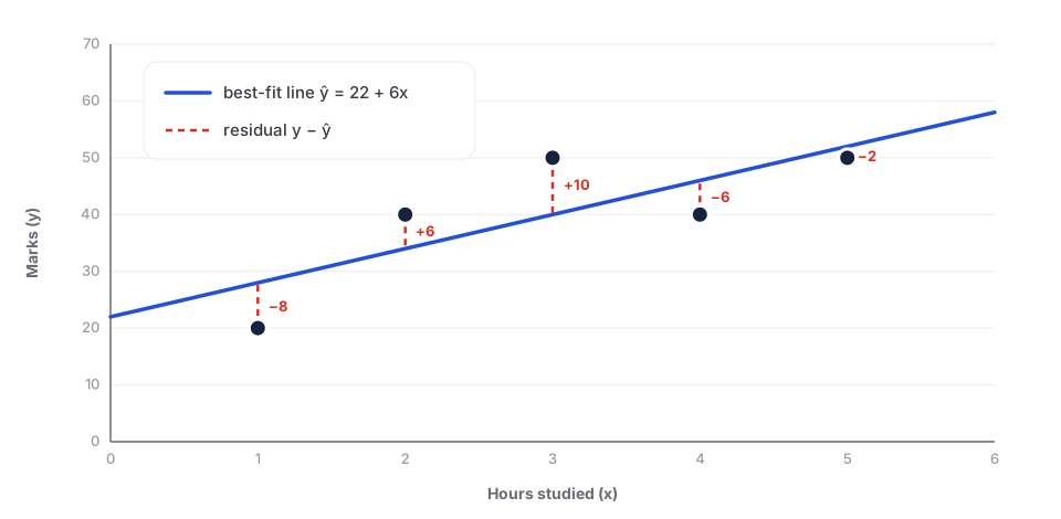
This method is called ordinary least squares (OLS). You'll see in the cost function lesson how this becomes a number we can minimise.
Solving It by Hand
For one feature, least squares has a neat closed-form answer:
Here and are the averages. Let's work it through.
Step 1: averages. and .
Step 2: a table of deviations.
| 1 | 20 | −2 | −20 | 40 | 4 |
| 2 | 40 | −1 | 0 | 0 | 1 |
| 3 | 50 | 0 | 10 | 0 | 0 |
| 4 | 40 | 1 | 0 | 0 | 1 |
| 5 | 50 | 2 | 10 | 20 | 4 |
| Sum | 60 | 10 |
Step 3: slope and intercept.
So the best-fit line is:
What the Numbers Mean
- Slope : every extra hour of study adds about 6 marks on average.
- Intercept : a student who studies 0 hours is predicted to get 22.
Be careful with the intercept. None of our students studied 0 hours, so 22 is just where the line happens to cross the axis, not a fact about non-studiers. In the same way, predicting for 20 hours gives 22 + 120 = 142 marks, which is impossible on a test out of 100. A line is only trustworthy inside the range of the data it learned from. Predicting outside it is called extrapolation, and it often goes wrong.
Fitting It With scikit-learn
Now let's check our hand calculation in code.
The Data as Arrays
import numpy as np
from sklearn.linear_model import LinearRegression

hours = np.array([1, 2, 3, 4, 5])
marks = np.array([20, 40, 50, 40, 50])
Passing a 1D Array by Mistake
Almost everyone does this the first time:
model = LinearRegression()
model.fit(hours, marks)ValueError: Expected 2D array, got 1D array instead:
array=[1 2 3 4 5].
Reshape your data either using array.reshape(-1, 1) if your data has a single feature or array.reshape(1, -1) if it contains a single sample.scikit-learn wants as a table: one row per example, one column per feature. hours is a flat list of 5 numbers, so we reshape it into 5 rows × 1 column. The -1 means "work out the number of rows for me".
X = hours.reshape(-1, 1)
print(X.shape)(5, 1)Training and Reading θ0 and θ1
model = LinearRegression()
model.fit(X, marks)

print("theta0 (intercept):", round(model.intercept_, 2))
print("theta1 (slope): ", round(model.coef_[0], 2))theta0 (intercept): 22.0
theta1 (slope): 6.0The same 22 and 6 we got by hand. Note that coef_ is an array, with one slope per feature. We have one feature, so we take coef_[0].
Predicting From the Line
print(model.predict([[6]]))
print(model.predict(X))[58.]
[28. 34. 40. 46. 52.]Check the first one by hand: . And here are the residuals for our five students:
| residual | |||
|---|---|---|---|
| 1 | 20 | 28 | −8 |
| 2 | 40 | 34 | 6 |
| 3 | 50 | 40 | 10 |
| 4 | 40 | 46 | −6 |
| 5 | 50 | 52 | −2 |
The residuals add up to exactly 0. That always happens with a least-squares line that has an intercept: the line sits right in the "middle" of the points.
Plotting It
import matplotlib.pyplot as plt

plt.scatter(hours, marks, color="black", label="students")
plt.plot(hours, model.predict(X), color="red", label="ŷ = 22 + 6x")
plt.xlabel("Hours studied")
plt.ylabel("Marks")
plt.legend()
plt.show()
Simple vs Multiple Linear Regression
| Simple | Multiple | |
|---|---|---|
| Features | One () | Many () |
| Equation | ||
| Shape | A line | A plane, or a "hyperplane" in more dimensions |
| Example | Marks from hours | Marks from hours, sleep and attendance |
The idea, the training and the scikit-learn code are the same. Only the number of columns in changes.
Where It's Used
- A first, quick model for any number you want to predict. Always try the simple thing first.
- Understanding a relationship: "how many extra sales per extra 1,000 taka of advertising?"
- Trend lines in business, economics and science.
- Add a sixth student who studied 6 hours and got 60 marks. Refit. Does the slope go up or down?
- Fit with
LinearRegression(fit_intercept=False). That forces the line through (0, 0). Compare the slope with 6. - Calculate the residuals with
marks - model.predict(X)and check they sum to 0.
The best-fit line is the one with the smallest sum of squared residuals. For our students it's ŷ = 22 + 6x.
Summary
- Simple linear regression fits .
- The best line minimises the sum of squared residuals (ordinary least squares).
- By hand: , then .
- In scikit-learn, must be 2D: use
reshape(-1, 1). - Next: the cost function, the single number that tells us how bad a line is.