Gradient Descent
Gradient descent is an algorithm that finds the minimum of a cost function by starting at a random point and repeatedly taking small steps downhill, in the direction where the cost falls fastest.
Your Path Through This Lesson
0 of 5 done
- Explain how the gradient tells you which way is downhill.
- Do one gradient descent step by hand.
- Choose a learning rate, and recognise one that's too big.
The Idea: Walking Down a Hill in Fog
Imagine you're standing somewhere on a hillside in thick fog. You can't see the valley, but you can feel the slope under your feet. A sensible plan:
- Feel which way the ground slopes down.
- Take a step that way.
- Repeat until the ground feels flat.
That's gradient descent. The hillside is the cost function bowl, your position is the current values of and , and "feeling the slope" means computing the gradient.
In the video we freeze at 22 so the bowl is a simple 2D curve. The real algorithm moves both parameters at once, but the idea is identical.
The Gradient Tells You the Way Down
The gradient is the slope of the cost function at your current point. It's just the derivative.
- If the slope is positive, the cost goes up to the right, so move left (decrease ).
- If the slope is negative, the cost goes up to the left, so move right (increase ).
- If the slope is zero, you're at the bottom. Stop.
In both cases you move against the slope. That's why there's a minus sign in the update rule.
The Update Rule
Repeat until the cost stops falling:
- means "update to". It's an assignment, not an equation.
- (alpha) is the learning rate: how big each step is.
- is the gradient for parameter .
For linear regression with , the derivatives work out to:
Notice the in the cost function has cancelled the 2 from the square. That was the whole reason for putting it there.
Update both parameters at the same time. Compute both gradients using the old and , then change both. If you update first and then use the new to compute 's gradient, you're doing a slightly different (and wrong) algorithm.
One Step by Hand
Same five students: hours 1 to 5, marks 20, 40, 50, 40, 50. Start at with learning rate .
Predictions are all 0, so the errors are −20, −40, −50, −40, −50.
Starting cost: .
Gradients:
Update:
New cost: the predictions are 8.6, 15.2, 21.8, 28.4, 35, which gives . One step, and the cost fell from 860 to about 190. Keep going and it slides all the way down to the minimum.
Gradient Descent in NumPy
import numpy as np

x = np.array([1, 2, 3, 4, 5])
y = np.array([20, 40, 50, 40, 50])
m = len(x)

def cost(t0, t1):
    return np.sum((t0 + t1 * x - y) ** 2) / (2 * m)

theta0, theta1 = 0.0, 0.0
alpha = 0.05
history = []

for i in range(5000):
    error = theta0 + theta1 * x - y
    grad0 = error.sum() / m
    grad1 = (error * x).sum() / m
    theta0, theta1 = theta0 - alpha * grad0, theta1 - alpha * grad1   # simultaneous update
    history.append(cost(theta0, theta1))

print(f"start cost:        {cost(0, 0):.1f}")
print(f"after 1 step:      {history[0]:.1f}")
print(f"theta0 = {theta0:.2f}, theta1 = {theta1:.2f}")
print(f"final cost: {history[-1]:.1f}")start cost: 860.0
after 1 step: 190.0
theta0 = 22.00, theta1 = 6.00
final cost: 24.0Gradient descent found θ0 = 22 and θ1 = 6, the same line we got by hand with least squares, and the same minimum cost of 24.
The Learning Rate α
The learning rate is the most important knob in gradient descent.
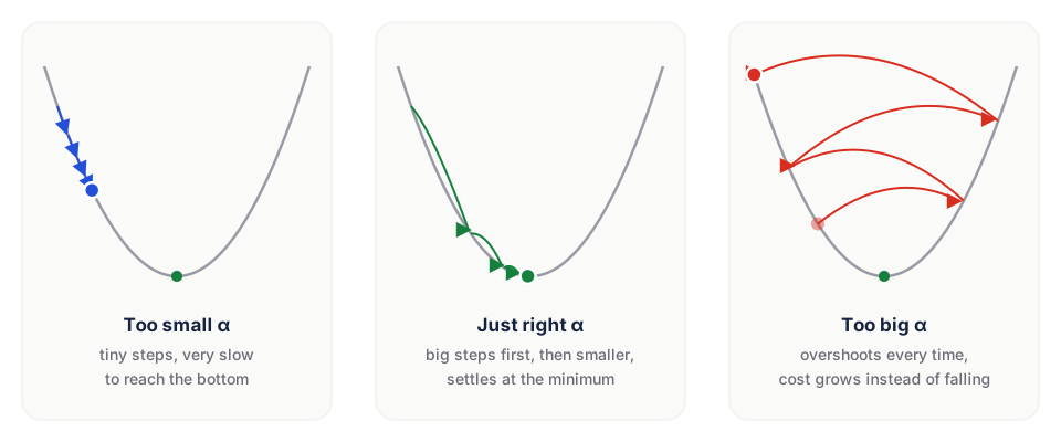
| Learning rate | What happens |
|---|---|
| Too small | Each step barely moves. It works, but takes forever. |
| Just right | Big steps at first, smaller ones as the bowl flattens, then it settles at the bottom. |
| Too big | Each step jumps right over the bottom to the other side, landing higher than before. The cost grows and the numbers explode. |
Why do the steps shrink on their own even with a fixed ? Because the step is gradient, and the gradient gets smaller as you approach the flat bottom.
Watching It Blow Up
Change one number, alpha = 0.2, and print the cost for the first three steps:
theta0, theta1, alpha = 0.0, 0.0, 0.2
for i in range(3):
    error = theta0 + theta1 * x - y
    theta0, theta1 = theta0 - alpha * error.sum() / m, theta1 - alpha * (error * x).sum() / m
print(f"step {i + 1}: cost = {cost(theta0, theta1):.1f}")step 1: cost = 1554.1
step 2: cost = 2851.6
step 3: cost = 5275.2The cost almost doubles every step. Let it run for 5000 steps and the numbers overflow to inf and nan. If your cost goes up, lower the learning rate first.
A common practical approach: try = 0.001, 0.01, 0.1 and so on, plot the cost against the iteration number for each, and pick the largest one where the curve still falls smoothly.
Gradient Descent vs the Formula
For simple linear regression we already had a formula (least squares). So why bother?
| Closed-form (least squares) | Gradient descent | |
|---|---|---|
| How | Solve one equation | Many small steps |
| Needs a learning rate? | No | Yes |
| Many features / huge data | Gets very slow | Scales well |
| Works for other models? | Only some | Almost everything, including neural networks |
scikit-learn's LinearRegression uses a direct solver. But almost every other model you'll meet, logistic regression and every neural network included, is trained with gradient descent or one of its cousins.
The Three Flavours
| Flavour | Gradient computed on | Trade-off |
|---|---|---|
| Batch | All examples each step | Smooth, but slow on big data. (That's what we wrote above.) |
| Stochastic (SGD) | One random example each step | Very fast, noisy path |
| Mini-batch | A small batch, e.g. 32 examples | The usual choice in deep learning |
Gradient descent is sensitive to the scale of the features. If one feature is in the thousands (salary) and another is between 0 and 1, the bowl becomes a long narrow valley and descent zig-zags slowly. Scale your features (e.g. with StandardScaler) before using it.
- Run the NumPy code with
alpha = 0.01and 5000 steps. Is it still at 22 and 6? Try 50,000 steps. - Plot
historywith matplotlib foralpha = 0.01andalpha = 0.05on the same chart. - Start from
theta0, theta1 = 100.0, -50.0. Does it still end at the same place? (It should: the bowl has only one bottom.)
Step against the gradient, scaled by the learning rate, and repeat until the cost stops falling.
Summary
- Gradient descent repeats until the cost stops falling.
- The gradient points uphill, so we step the opposite way.
- The learning rate controls step size: too small is slow, too big diverges.
- On our data it reaches the same line as least squares: .
- Next: how do we say how good that line is? With R squared.