R Squared and Adjusted R Squared

R squared (R²) tells you what fraction of the variation in the target your model explains. Adjusted R² does the same, but penalises you for adding features that don't really help.

By the End of This Lesson You Can

Explain R² as the share of variation a model explains.
Compute R² and adjusted R² by hand and in code.
Say why adjusted R² is fairer when comparing models.

The Question R² Answers

We have our line, $y^= 22 + 6 x$ . Is it any good? The cost was 24, but "24" means nothing on its own. Is that good? Bad? It depends on the units, and it changes if you measure marks out of 100 or out of 1,000.

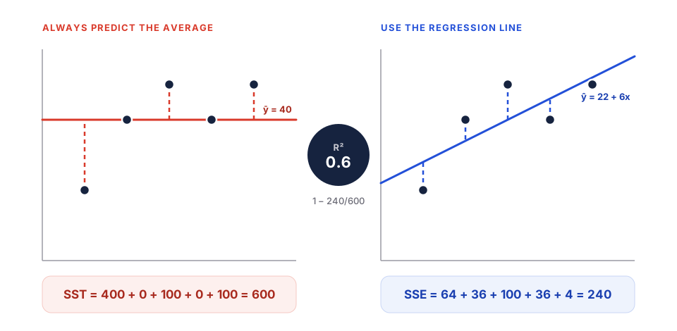
R² fixes that by comparing your model with the laziest possible model: one that ignores $x$ completely and always predicts the average, $y ˉ$ .

If your model is no better than predicting the average, R² = 0.
If your model is perfect, R² = 1.
Everything in between tells you how much of the "spread" in $y$ your model accounts for.

Two Kinds of Error

Total sum of squares (SST) is the error of the lazy, average-only model:

S S_{tot} = \sum (y_{i} - y ˉ)^{2}

Residual sum of squares (SSE) is the error that's left over after your model:

S S_{res} = \sum (y_{i} - y^_{i})^{2}

Then:

R^{2} = 1 - \frac{S S _{res}}{S S _{tot}}

Read it as: "the fraction of the original error that the model got rid of."

SST is the error of always predicting the average. SSE is the error left after the regression line. R² is the share of SST that the line removed.

Working It Out by Hand

Our five students again, with $y ˉ = 40$ and the line $y^= 22 + 6 x$ :

$x$	$y$	$y - y ˉ$	$(y - y ˉ)^{2}$	$y^$	$y - y^$	$(y - y^)^{2}$
1	20	−20	400	28	−8	64
2	40	0	0	34	6	36
3	50	10	100	40	10	100
4	40	0	0	46	−6	36
5	50	10	100	52	−2	4
		SST	600		SSE	240

R^{2} = 1 - \frac{240}{600} = 1 - 0.4 = 0.6

Our line explains 60% of the variation in marks. The other 40% comes from things the line doesn't know about: sleep, how hard the test was, luck, and so on.

Checking It in Code

python

import numpy as np
from sklearn.linear_model import LinearRegression
from sklearn.metrics import r2_score

X = np.array([1, 2, 3, 4, 5]).reshape(-1, 1)
y = np.array([20, 40, 50, 40, 50])

model = LinearRegression().fit(X, y)
y_pred = model.predict(X)

print("R2 :", round(r2_score(y, y_pred), 4))
print("R2 :", round(model.score(X, y), 4))   # same thing, built into the model

Output

R2 : 0.6
R2 : 0.6

Watch Out

The argument order is r2_score(y_true, y_pred): the real answers first. Swap them and you get a different, wrong number with no error message.

Reading the Value

R²	What it means
1.0	Perfect: every point is exactly on the line. On real data, this usually means a bug or leakage.
0.6	The model explains 60% of the variation.
0.0	No better than always predicting the average.
below 0	Worse than always predicting the average.

Yes, R² can be negative. That surprises a lot of people because of the "squared" in the name. A model that always predicts 0 marks would have $S S_{res} = 8600$ , so $R^{2} = 1 - 8600/600 \approx - 13.3$ . On the test set, a badly overfitted model can easily score below zero.

Note

What counts as a "good" R² depends on the field. In physics experiments you might expect 0.99. For predicting human behaviour, like sales or exam marks, 0.5 can be genuinely useful. Always compare against a sensible baseline rather than a magic number.

The Problem With R²

Here's the catch: R² never goes down when you add a feature. Even a completely useless one, like each student's roll number or a column of random numbers, will nudge R² up a little, because the model can always use it to fit the training data slightly better by chance.

So if you judge only by R², you'll keep adding junk features and think you're improving.

Adjusted R²

Adjusted R² adds a penalty for every extra feature:

R_{adj}^{2} = 1 - \frac{( 1 - R ^{2} ) ( n - 1 )}{n - p - 1}

$n$ = number of examples (rows)
$p$ = number of features (columns)

For our data, $n = 5$ and $p = 1$ :

R_{adj}^{2} = 1 - \frac{( 1 - 0.6 ) ( 5 - 1 )}{5 - 1 - 1} = 1 - \frac{0.4 \times 4}{3} \approx 0.4667

It's lower than 0.6 because with only five students, one feature is already "expensive". Adjusted R² rises only if a new feature improves the fit more than you'd expect by chance. If you add a junk feature, it goes down.

python

n, p = X.shape
r2 = r2_score(y, y_pred)
adj_r2 = 1 - (1 - r2) * (n - 1) / (n - p - 1)
print("Adjusted R2:", round(adj_r2, 4))

Output

Adjusted R2: 0.4667

scikit-learn doesn't have a built-in function for adjusted R², so this one-liner is how everyone computes it.

R² vs Adjusted R²

	R²	Adjusted R²
Adding a useless feature	Goes up (slightly)	Goes down
Adding a useful feature	Goes up	Goes up
Can be compared across models with different numbers of features?	Not fairly	Yes
Always ≤ R²?		Yes

Try It Yourself

Add a column of random numbers as a second feature: X2 = np.column_stack([X, np.random.rand(5)]). Fit again. Did R² go up? Compute adjusted R² with $p = 2$ . What happened?
Compute R² on a model that always predicts 40 (the mean). You should get exactly 0.
Why can't you compute adjusted R² when $n = p + 1$ ?

The Key Idea

R² = 1 − SSE / SST. Adjusted R² adds a penalty for every extra feature.

Summary

$R^{2} = 1 - S S_{res} / S S_{tot}$ : the share of variation the model explains.
For our line, $R^{2} = 1 - 240/600 = 0.6$ .
R² can be negative, and it never falls when you add features, even useless ones.
Adjusted R² penalises extra features: for us, about 0.4667.
Next up in this part: MSE, MAE and RMSE, the error metrics that keep the target's units.

Your Path Through This Lesson

The Question R² Answers

Two Kinds of Error

Working It Out by Hand

Checking It in Code

Reading the Value

The Problem With R²

Adjusted R²

R² vs Adjusted R²

Summary